Pollination Algorithm 2.0 Mastery: Blooming Success with Nature’s Precision

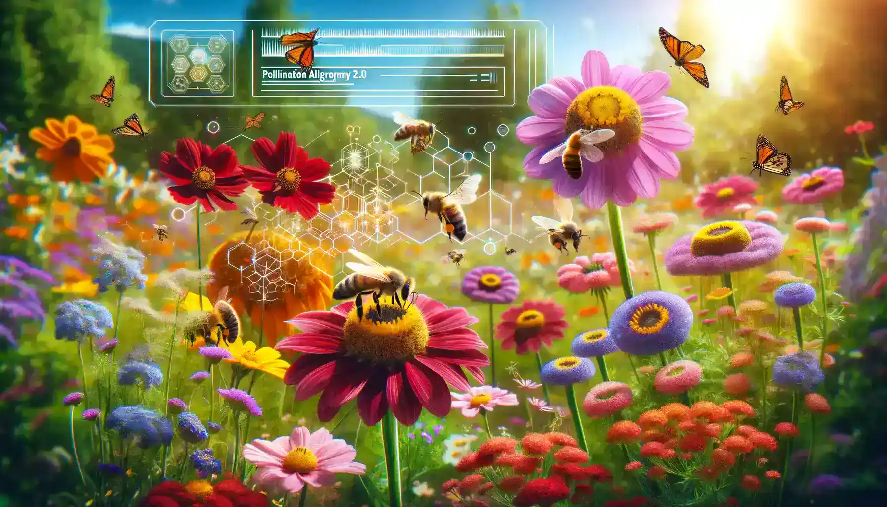
Every time a bee drifts from one flower to the next, it’s running an optimization problem: where’s the next best source of nectar, and what’s the most efficient path to get there? A pollination algorithm takes that exact behavior and turns it into maths, a way to search huge, messy solution spaces without getting stuck on the first decent answer it finds.

Originally formalized as the Flower Pollination Algorithm (FPA) by Xin-She Yang in 2012, this approach has since been extended, hybridized, and tuned into what’s often referred to informally as Pollination Algorithm 2.0, versions that fix the convergence problems of the original and add adaptive, learning-driven components. This guide breaks down how it works, where it’s actually used, and how you can implement it yourself.

What Is a Pollination Algorithm?

At its core, this is a metaheuristic optimization technique, meaning it doesn’t guarantee the perfect answer, but it finds very good answers to problems that are too complex to solve exhaustively. It belongs to the same family as genetic algorithms, ant colony optimization, and particle swarm optimization: all borrow rules from biological systems that are already good at exploring and exploiting resources efficiently.

The core idea is a split between two pollination types found in nature:

• Global pollination (biotic, cross-pollination): pollen travels long distances, carried by insects, birds, or wind, modeled mathematically using Lévy flights, which allow occasional large jumps across the search space
• Local pollination (abiotic, self-pollination): pollination happens between nearby flowers of the same plant, modeled as small, local adjustments between existing candidate solutions

A parameter called the switch probability decides, at each step, whether to explore globally or refine locally. That balance between exploration and exploitation is what makes a pollination algorithm effective on problems where a pure hill-climbing approach would get trapped on a mediocre solution.

How It Actually Works

Every implementation runs the same six-step loop, repeated generation after generation until the population converges. Here’s what happens at each stage.

Step 1: Initialize the Population

The process starts by generating a set of candidate solutions, the “flowers”, scattered randomly across the search space. Each one is just a possible answer to the problem, with no information yet about which is any good.

Step 2: Evaluate Fitness

Every candidate is scored against a fitness function, the equivalent of asking “how good is this flower at attracting pollinators?” This score is what everything else in the loop is built around.

Step 3: Choose Global or Local Pollination

For each solution, the switch probability decides its fate: a coin flip weighted toward global or local search, depending on how that probability is tuned.

Step 4: Update Solutions

This is where the actual movement happens:

• Global pollination: the solution takes a Lévy flight step toward the current best solution, a jump that’s usually small but occasionally large, letting the search escape local traps
• Local pollination: the solution blends with two other randomly chosen solutions from the population, making a smaller, more conservative adjustment

Step 5: Re-Evaluate and Keep the Best

Updated solutions are scored again. Anything that improved replaces the old version; anything worse gets discarded. The population only ever moves toward better fitness, never backward.

Step 6: Repeat Until Convergence

Steps 2 through 5 are repeated until the population converges on a stable solution or a stopping condition – a fixed number of generations, a fitness threshold, or a time budget – is reached.

In pseudocode, the whole loop looks like this:

Initialize population of n flowers with random solutions Evaluate fitness of each flower Find the current best solution g* while (stopping condition not met): for each flower i in population: if rand() < switch_probability: # Global pollination x_i = x_i + LevyFlight() * (g* - x_i) else: # Local pollination pick two random flowers j, k from population x_i = x_i + rand() * (x_j - x_k) Evaluate fitness of updated x_i if new fitness is better: keep updated x_i else: keep original x_i Update g* if a better solution was found

This is what separates a pollination algorithm from simpler search methods: it never fully commits to greedy, purely local search, nor does it waste all its effort on random global jumps. The switch probability keeps both mechanisms running side by side.

The Evolution to 2.0

The original FPA had known weaknesses: it could converge prematurely on suboptimal solutions, and its performance was sensitive to how the switch probability was tuned. What’s commonly referred to as Pollination Algorithm 2.0 isn’t a single official release; it’s the collective set of improvements researchers have layered onto the base method over time. These typically include:

• Adaptive switch probability that changes dynamically as the search progresses, rather than staying fixed
• Hybridization with other metaheuristics, such as particle swarm optimization or differential evolution, to combine strengths
• Machine learning-guided parameter tuning, where a model learns which settings work best for a given problem class
• Chaotic maps used in place of purely random number generation, improving diversity in the search space

Together, these refinements make the modern version noticeably more reliable on large, high-dimensional problems than the original 2012 formulation, with faster convergence, fewer wasted iterations, and better resistance to getting stuck.

How It Compares to Other Nature-Inspired Optimizers

Approach	Core Mechanism	Strengths	Weaknesses
Pollination Algorithm	Global (Lévy flight) vs. local pollination, governed by switch probability	Strong exploration-exploitation balance; few tunable parameters	Can be sensitive to switch probability if not adaptive
Genetic Algorithm	Selection, crossover, mutation across generations	Well-studied, works on discrete and combinatorial problems	Can converge slowly; needs careful crossover/mutation tuning
Particle Swarm Optimization	Particles adjust velocity based on personal and swarm-best positions	Fast convergence on continuous problems	Prone to premature convergence without diversity control
Ant Colony Optimization	Pheromone trails reinforce good paths over iterations	Excellent for routing and graph-based problems	Computationally heavier for large graphs

Real-World Use Cases

Logistics and route optimization: This approach can search delivery route permutations far faster than brute force, balancing distance, fuel cost, and delivery windows.

Portfolio and resource allocation: In finance and operations, it helps allocate limited resources (capital, compute, and inventory) across competing priorities to maximize a defined return.

Swarm robotics: Coordinating multiple robots toward a shared goal like warehouse picking or search-and-rescue coverage maps naturally maps onto the same global/local search logic this method uses.

Neural network hyperparameter tuning: Instead of grid search, teams increasingly use a pollination algorithm to search for learning rate, batch size, and architecture choices more efficiently.

AI tools

TensorFlow – Ideal for implementing machine learning models, TensorFlow provides a comprehensive platform for building and deploying Pollination Algorithm 2.0 applications.

PyTorch – Similar to TensorFlow, PyTorch is a popular deep-learning library that can be employed for developing and training advanced algorithms, including Pollination Algorithm 2.0.

Scikit-learn – This versatile machine-learning library is valuable for implementing various algorithms, including those related to optimization and precision, offering tools for data preprocessing, model selection, and evaluation.

Jupyter Notebooks – Jupyter Notebooks provide an interactive and collaborative environment for running Python code. They are excellent for experimenting with algorithms, visualizing data, and sharing insights.

Pandas – For data manipulation and analysis, Pandas is a powerful Python library. It can help preprocess and organize data sets, a crucial step in the development and training of precision-focused algorithms.

Matplotlib and Seaborn – These visualization libraries are essential for creating plots and graphs, aiding in the interpretation and communication of results obtained from Pollination Algorithm 2.0 applications.

Google Colab – Offering a cloud-based environment with free access to GPUs, Google Colab is suitable for running resource-intensive algorithms, enabling users to harness significant computing power for training sophisticated models.

IBM Watson Studio – For a comprehensive AI development and deployment environment, IBM Watson Studio provides tools for data scientists, developers, and domain experts, facilitating the creation of intelligent applications.

Conclusion

A pollination algorithm takes something nature already solved- efficient, decentralized search for the best available resource – and turns it into a practical optimization tool. The original FPA laid the groundwork; the adaptive, hybridized techniques grouped under “version 2.0” address its early weaknesses and extend it to harder, higher-dimensional problems.

Whether you’re optimizing delivery routes, tuning a model, or coordinating a robotic swarm, it’s worth having in your optimization toolkit alongside genetic algorithms and particle swarm methods, not as a replacement, but as another option suited to specific kinds of problems.

FAQs